Matrix Addressing

Overview

Finite-volume discretisation produces a sparse linear system \(A \mathbf{x} = \mathbf{b}\) where each row corresponds to a mesh cell and each non-zero off-diagonal entry corresponds to a face shared by two cells. NeoN assembles this system in three parts:

• Local system matrix — all cell-to-cell connections within the current MPI rank.

• Physical-boundary matrix — contributions from Dirichlet/Neumann boundaries.

• Processor-boundary matrix — contributions from faces shared with neighbouring MPI ranks.

The central object that links mesh topology to matrix storage is FaceToMatrixAddress (include/NeoN/linearAlgebra/faceToMatrixAddress.hpp). It stores three compact offset arrays (diagOffset, ownerOffset, neighbourOffset) that map every mesh face to a position inside the flat values array of the corresponding matrix.

Further details:

• FaceToMatrixAddress

• LinearSystem

Currently, only two matrix formats are supported: CSR and COO. These are hardcoded, with the system matrix stored in CSR format and the boundary matrix stored in COO format.

CSR Format

The local system matrix is stored in Compressed Sparse Row (CSR) format via CsrSparsityPattern (include/NeoN/linearAlgebra/csrSparsityPattern.hpp):

Vector<IndexType> rowOffs_;   // size nCells + 1
Vector<IndexType> colIdxs_;   // size nnz (number of non-zeros)
// values stored separately in Matrix::values_

rowOffs[i+1] - rowOffs[i] gives the number of non-zeros in row i. Iterating over row i:

for (localIdx k = rowOffs[i]; k < rowOffs[i+1]; ++k)
{
    // colIdxs[k] is the column index
    // values[k]  is A[i, colIdxs[k]]
}

Row Layout and Face Addressing Arrays

Within every row of a matrix A the non-zero values are stored in row-major order. This leads to entries being sorted as lower | diag | upper in a row as shown below:

Row i: [ A[i,j0] ... A[i,j_{k-1}] | A[i,i] | A[i,j_{k+1}] ... A[i,j_{m}] ]
       |<----- lower (j < i) ----->|<-diag->|<----- upper (j > i) -------->|

diagOffset[i] equals the count of lower-triangular entries in row i, which is also the number of internal faces for which cell i is the neighbour (i.e. has a larger index than the owner). Additionally, the FaceToMatrixAddress class stores ownerOffset[i] and neighbourOffset[i], which map from a given face ID to the offset of a lower or upper matrix element, respectively. Note that by construction ownerOffset[i] and neighbourOffset[i] map to the upper triangular and lower triangular matrix respectively. These face addressing arrays are stored as uint8_t arrays. The following table gives as summary

Mesh - Matrix Example

Mesh Topology

Consider the following 1-D mesh partitioned into 2 parts with 4 cells (Ci) on each rank 0

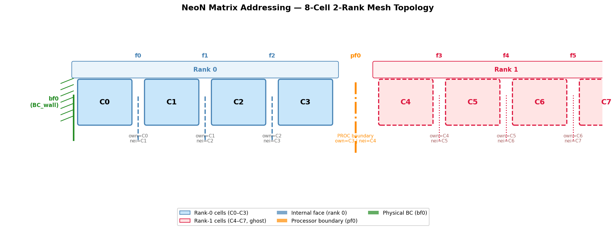
Generated by generate_matrix_addressing_figure.py. Rank-0 cells (blue) and rank-1 cells (red, shown as ghost). Internal faces f0–f2 are on rank 0; pf0 is the processor boundary; bf0 is a wall.

Face list for rank 0:

• Internal faces (rank 0): f0 (own=C0, nei=C1), f1 (own=C1, nei=C2), f2 (own=C2, nei=C3)

• Physical boundary face: bf0 — left wall of C0

• Processor boundary face: pf0 — right side of C3, shared with rank 1 (own=C3, remote=C4)

The local matrix on rank 0 has shape 4×4 with 10 non-zeros (2 entries per interior face + 4 diagonals).

Matrix Sparsity Pattern

The resulting sparsity pattern of the local system matrix, i.e. the position of the non zero entries is shown in the figure below.

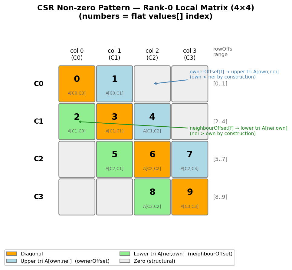
Generated by generate_matrix_addressing_figure.py. Numbers show the flat values[] index. Orange = diagonal, blue = upper triangular A[own,nei] (via ownerOffset), green = lower triangular A[nei,own] (via neighbourOffset).

For the simple 1d mesh the resulting local system matrix is banded with single lower and upper off-diagonal band.

Construction Walkthrough

The procedure to construct the sparsity pattern and corresponding offsets is implemented in the setSparsityPatternFaceToMatrixAddressSerial function (see src/linearAlgebra/faceToMatrixAddress.cpp). It builds the arrays in five passes:

Step 1 — count non-zeros per cell (initialised to 1 for the diagonal):

Iterate all faces and increment the count for each owner and neighbour cell.

nFacesPerCell = [1, 1, 1, 1]
f0: nFacesPerCell[C0]++, nFacesPerCell[C1]++  → [2, 2, 1, 1]
f1: nFacesPerCell[C1]++, nFacesPerCell[C2]++  → [2, 3, 2, 1]
f2: nFacesPerCell[C2]++, nFacesPerCell[C3]++  → [2, 3, 3, 2]

Step 2 — compute row offsets (exclusive prefix sum):

From the face per cell count the rowOffsets can be computed as a prefix sum.

rowOffs = [0, 2, 5, 8, 10]

Step 3 — assign lower-triangular positions (nFacesPerCell reset to 0):

For each face, the neighbour cell receives a new position for the column=own entry. Because nei > own, this column is in the lower triangle of the neighbour’s row:

f0: segIdx = nFacesPerCell[C1]++ = 0 → neighbourOffset[f0] = 0, colIdx[2+0] = C0
f1: segIdx = nFacesPerCell[C2]++ = 0 → neighbourOffset[f1] = 0, colIdx[5+0] = C1
f2: segIdx = nFacesPerCell[C3]++ = 0 → neighbourOffset[f2] = 0, colIdx[8+0] = C2

Step 4 — place diagonal:

Once all lower diagonal entries are know the diagonal offset can be updated

C0: diagOffset[C0] = nFacesPerCell[C0] = 0, colIdx[0+0] = C0, nFacesPerCell[C0]++ = 1
C1: diagOffset[C1] = nFacesPerCell[C1] = 1, colIdx[2+1] = C1, nFacesPerCell[C1]++ = 2
C2: diagOffset[C2] = nFacesPerCell[C2] = 1, colIdx[5+1] = C2, nFacesPerCell[C2]++ = 2
C3: diagOffset[C3] = nFacesPerCell[C3] = 1, colIdx[8+1] = C3, nFacesPerCell[C3]++ = 2

Step 5 — assign upper-triangular positions (positions start after the diagonal):

For each face, the owner cell receives a new position for the column=nei entry. Because own < nei, this column is in the upper triangle of the owner’s row:

f0: segIdx = nFacesPerCell[C0]++ = 1 → ownerOffset[f0] = 1, colIdx[0+1] = C1
f1: segIdx = nFacesPerCell[C1]++ = 2 → ownerOffset[f1] = 2, colIdx[2+2] = C2
f2: segIdx = nFacesPerCell[C2]++ = 2 → ownerOffset[f2] = 2, colIdx[5+2] = C3

Resulting Arrays

Array	Values	Notes
rowOffs	[0, 2, 5, 8, 10]	size = nCells+1 = 5
colIdxs	[0, 1, 0, 1, 2, 1, 2, 3, 2, 3]	size = nnz = 10
diagOffset	[0, 1, 1, 1]	one entry per cell (C0..C3)
ownerOffset	[1, 2, 2]	f0,f1,f2 → upper tri A[own,nei]
neighbourOffset	[0, 0, 0]	f0,f1,f2 → lower tri A[nei,own]

Why ownerOffset → upper triangular

By construction, NeoN guarantees owner[f] < neighbour[f] for every internal face f. This means that in the owner’s row (row index = own), the column that points to the neighbour has column index nei > own — which is the upper triangle. Conversely, in the neighbour’s row (row index = nei), the column pointing back to the owner has column index own < nei — which is the lower triangle. This invariant is what makes ownerOffset the upper-triangular offset and neighbourOffset the lower-triangular offset.

LDU to CSR Correspondence

In comparison OpenFOAM’s classical LDU format stores three separate arrays: diag, lower, and upper. NeoN encodes the same information in a single values array. The mapping for the 4-cell rank-0 example is:

LDU concept	NeoN access	Flat index
diag[C0]	values[diagIdx(C0)]	0
upper[f0] = A[C0,C1]	values[upperIdx(C0, f0)]	1
lower[f0] = A[C1,C0]	values[lowerIdx(C1, f0)]	2
diag[C1]	values[diagIdx(C1)]	3
upper[f1] = A[C1,C2]	values[upperIdx(C1, f1)]	4
lower[f1] = A[C2,C1]	values[lowerIdx(C2, f1)]	5
diag[C2]	values[diagIdx(C2)]	6
upper[f2] = A[C2,C3]	values[upperIdx(C2, f2)]	7
lower[f2] = A[C3,C2]	values[lowerIdx(C3, f2)]	8
diag[C3]	values[diagIdx(C3)]	9

The Laplacian kernel illustrates the canonical addressing pattern (symmetric operator, flux = deltaCoeffs * gamma * magSf > 0):

auto own = faceOwner[facei];
auto nei = faceNeighbour[facei];

// A[nei, own] — lower triangular, in neighbour's row:
values[rowOffs[nei] + neighbourOffset[facei]] += flux;
// values[lowerIdx(nei, facei)] += flux;   // equivalent via matrixIterator

// A[own, nei] — upper triangular, in owner's row:
values[rowOffs[own] + ownerOffset[facei]] += flux;
// values[upperIdx(own, facei)] += flux;   // equivalent via matrixIterator

// Diagonal — flux leaves each cell (symmetric → same magnitude for own and nei):
Kokkos::atomic_sub(&values[rowOffs[own] + diagOffset[own]], flux);
Kokkos::atomic_sub(&values[rowOffs[nei] + diagOffset[nei]], flux);

The divergence operator uses the same addressing but different signs on the off-diagonals and diagonal (asymmetric); see Operator Assembly for details.

Physical Boundary Contributions (COO)

A boundary face touches only one cell — the owner. Its contribution modifies the diagonal of that cell’s row and the right-hand side. No off-diagonal coupling in the system matrix is introduced, so a full CSR row is unnecessary.

NeoN stores physical boundary contributions in a CooSparsityPattern class (include/NeoN/linearAlgebra/cooSparsityPattern.hpp):

• rowOffs[bfacei] = owner cell index

• colIdx[bfacei] = celli + diagOffset[celli] (see note below)

Built in setBoundarySparsityPattern (faceToMatrixAddress.cpp):

// For boundary face bfacei touching owner cell celli:
bColIdx[bfacei] = celli + diagOffset[celli];
bRowIdx[bfacei] = celli;

For the 8-cell example (bf0 → C0):

bRowIdx = [0]    (owner cell = C0 = 0)
bColIdx = [0]    (= C0 + diagOffset[C0] = 0 + 0 = 0)

Note

The colIdx formula uses celli + diagOffset[celli], not the full flat CSR index rowOffs[celli] + diagOffset[celli]. The two are equal only for cell 0. This value is a bookkeeping tag, not a direct index into matrix_.values(). Physical boundary contributions are written directly to the CSR diagonal inside the operator kernels (e.g. computeLaplacianBoundImpl); the COO boundaryMatrix_ tracks the face-to-cell mapping for other purposes. Do not use bColIdx as a flat CSR offset.

Processor Boundary Contributions (COO)

A processor boundary face couples a cell on the local rank to a cell on a neighbouring rank. The remote cell’s value is not stored locally; it arrives via MPI. After the exchange, the received contribution is subtracted from the diagonal of the local owner cell.

The sparsity is again COO, built in setProcBoundarySparsityPattern (faceToMatrixAddress.cpp):

// For proc-boundary face bfacei touching local cell celli:
pColIdx[bfacei] = celli + diagOffset[celli];
pRowIdx[bfacei] = celli;

For the 8-cell example (pf0 → C3):

pRowIdx = [3]    (owner cell = C3 = 3)
pColIdx = [4]    (= C3 + diagOffset[C3] = 3 + 1 = 4)

The MPI exchange happens in LinearSystem::communicate() (linearSystem.hpp):

1. Copy processor-boundary values to send buffer.

2. MPI_Alltoallv exchanges contributions with all neighbouring ranks.

3. Subtract received values from the local CSR matrix diagonal via sub(recvBuffer, boundaryMatrixMap, matrix_.values()).

Note

pColIdx = celli + diagOffset[celli] is a bookkeeping tag (not a flat CSR offset), same as the physical-boundary case. LinearSystem::communicate() does not use this colIdx directly; instead it calls computeRowToDiagonalMap which correctly resolves rowOffs[cell] + diagOffset[cell] at scatter time. CommunicationPattern::boundaryMapVector is currently unused (see FIXME in unstructuredMesh.cpp).

How to Access Values in Practice

auto mi     = ls.faceToMatrixAddress();    // FaceToMatrixAddress
auto values = ls.matrix().values().view(); // flat values array

// 1. Diagonal of cell i:
values[mi->diagIdx(i)] += contribution;

// 2. A[own, nei] (upper triangular) for internal face f:
values[mi->upperIdx(own, f)] += contribution;
// Equivalent direct form: values[rowOffs[own] + ownerOffset[f]] += contribution;

// 3. A[nei, own] (lower triangular) for internal face f:
values[mi->lowerIdx(nei, f)] += contribution;
// Equivalent direct form: values[rowOffs[nei] + neighbourOffset[f]] += contribution;

// 4. Physical boundary contribution:
//    Operator kernels (e.g. computeLaplacianBoundImpl) write directly to
//    the CSR diagonal and RHS — there is no automatic scatter from boundaryMatrix.
auto own = faceCells[bcFaceIdx];
Kokkos::atomic_sub(&values[mi->diagIdx(own)], diagonalContribution);
rhs[own] -= rhsContribution;